Introduction
tidymodels is the new framework from Max Kuhn, David Vaughan, and Julia Silge at RStudio. It’s the successor to the caret package, which was heavily featured in Max Kuhn’s book Applied Predictive Modeling.
tidymodels promises a modular, extensible design for machine learning in R. It also has a wonderful website design to help you get started as soon as possible, with a focus on examples and case studies walking you through the components of the platform.
In this article, I want to translate concepts between tidymodels and scikit-learn, Python’s standard machine learning ecosystem. I hope this will be useful for Python Data Scientists interested in R, and R users who want to learn a little more about Python.
I’ll cover the key machine learning workflows with scikit-learn and tidymodels side-by-side, starting with preprocessing and feature engineering, model tranining and cross-validation, as well as evaluation and comparison.
I think you’ll find that while both frameworks have their own unique advantages, there are many conceptual similarities that have helped me understand both frameworks better.
tidymodels and sklearn
We’ll go through this tidymodels example: 4 Tune Model Parameters side-by-sideline with sklearn.
Notebook saved here: https://github.com/tmastny/sageprocess/blob/master/vignettes/sklearn-tidymodels-example1.ipynb
tidymodels
library(tidymodels)
library(modeldata)
library(vip)
library(readr)

cells <- read_csv("cells.csv")
sklearn
import pandas as pd
import numpy as np

np.random.seed(753)
cells = pd.read_csv("cells.csv")
cell_split <- initial_split(
cells,
strata = class
)
cell_train <- training(cell_split)
cell_test <- testing(cell_split)from sklearn.model_selection import train_test_split
features = cells.drop('class', axis=1)
outcome = cells['class']
X_train, X_test, y_train, y_test = train_test_split(
features,
outcome,
test_size=0.25,
stratify=outcome
)We have to do a little preprocessing. All the features are numeric,
but the outcome is binary. R expects categorical outcomes as factors.
Python automatically changes outcome strings with LabelBinarizer.
We also use the identity transformation FunctionTransformer() to remove
the case column by dropping it from selected columns.
tree_rec <- recipe(class ~ ., data = cells) %>%
  step_rm(case) %>%
  step_string2factor(all_outcomes())
from sklearn.preprocessing import FunctionTransformer
from sklearn.compose import make_column_transformer
tree_preprocess = make_column_transformer(
(FunctionTransformer(), features.drop('case', axis=1).columns)
)With R, we chose the implementation using set_engine and set_mode.
For sklearn, if we wanted a different implementation we would import
a different module that implemented the sklearn interface.
tree_model <- decision_tree(
  cost_complexity = tune(),
  tree_depth = tune()
) %>%
  set_engine("rpart") %>%
  set_mode("classification")
from sklearn.tree import DecisionTreeClassifierBoth frameworks have a way to combine all the components of the model.
set.seed(345)

tree_wf <- workflow() %>%
  add_model(tree_model) %>%
  add_recipe(tree_rec)
from sklearn.pipeline import make_pipeline
tree_pipeline = make_pipeline(
tree_preprocess,
DecisionTreeClassifier()
)Next, we can come up with tuning grids. tidymodels has sensible defaults for all parameters. With sklearn, you typically have to come up with them yourself.
tree_grid <- grid_regular(
  cost_complexity(),
  tree_depth(),
  levels = 5
)

tree_grid
## # A tibble: 25 x 2
## cost_complexity tree_depth
## <dbl> <int>
## 1 0.0000000001 1
## 2 0.0000000178 1
## 3 0.00000316 1
## 4 0.000562 1
## 5 0.1 1
## 6 0.0000000001 4
## 7 0.0000000178 4
## 8 0.00000316 4
## 9 0.000562 4
## 10 0.1 4
## # … with 15 more rowsparam_grid = {
'decisiontreeclassifier__max_depth': [1, 4, 8, 11, 15],
'decisiontreeclassifier__ccp_alpha': [
0.0000000001, 0.0000000178, 0.00000316, 0.000562, 0.1
]
}Next, we construct and run cross-validation. By default, tidymodels calculates both accuracy and area under the ROC curve. We’ll need to add those manually to sklearn’s metrics.
set.seed(234)
cell_folds <- vfold_cv(cell_train, v = 5)

tree_res <- tree_wf %>%
  tune_grid(
    resamples = cell_folds,
    grid = tree_grid
  )
from sklearn.model_selection import GridSearchCV
from sklearn.metrics import make_scorer
from sklearn.metrics import accuracy_score
from sklearn.metrics import roc_auc_score
tree_scorer = {
'roc_auc': make_scorer(roc_auc_score, needs_proba=True),
'accuray': make_scorer(accuracy_score)
}
tree_tuner = GridSearchCV(
tree_pipeline, param_grid, cv=5,
scoring=tree_scorer,
refit='roc_auc'
)
tree_res = tree_tuner.fit(X_train, y_train)List training metrics and hyperparamterics.
best_param <- tree_res %>%
  select_best("roc_auc")

best_param
## # A tibble: 1 x 3
## cost_complexity tree_depth .config
## <dbl> <int> <fct>
## 1 0.0000000001 4 Model06tree_res.best_params_## {'decisiontreeclassifier__ccp_alpha': 1.78e-08, 'decisiontreeclassifier__max_depth': 4}tree_res %>%
show_best("roc_auc")## # A tibble: 5 x 8
## cost_complexity tree_depth .metric .estimator mean n std_err .config
## <dbl> <int> <chr> <chr> <dbl> <int> <dbl> <fct>
## 1 0.0000000001 4 roc_auc binary 0.862 5 0.00578 Model06
## 2 0.0000000178 4 roc_auc binary 0.862 5 0.00578 Model07
## 3 0.00000316 4 roc_auc binary 0.862 5 0.00578 Model08
## 4 0.000562 4 roc_auc binary 0.862 5 0.00578 Model09
## 5 0.0000000001 8 roc_auc binary 0.846 5 0.0105 Model11pd.DataFrame(tree_res.cv_results_) \
.sort_values('mean_test_roc_auc', ascending=False) \
.rename(columns={
'param_decisiontreeclassifier__ccp_alpha': 'cost',
'param_decisiontreeclassifier__max_depth': 'max_depth'
}) \
[[
'cost', 'max_depth',
'mean_test_accuray', 'mean_test_roc_auc'
]] \
.head(5)## cost max_depth mean_test_accuray mean_test_roc_auc
## 6 1.78e-08 4 0.797240 0.839899
## 1 1e-10 4 0.796584 0.839053
## 11 3.16e-06 4 0.795257 0.837103
## 16 0.000562 4 0.795917 0.837055
## 0 1e-10 1 0.738461 0.779942Variable importance. This is where sklearn becomes significantly more difficult. Column name metadata is not saved in the final output, so we have to manually add column names back to an ordered list of feature importances.
best_tree <- tree_wf %>%
  finalize_workflow(best_param) %>%
  fit(data = cell_train)

best_tree %>%
  pull_workflow_fit() %>%
  vip()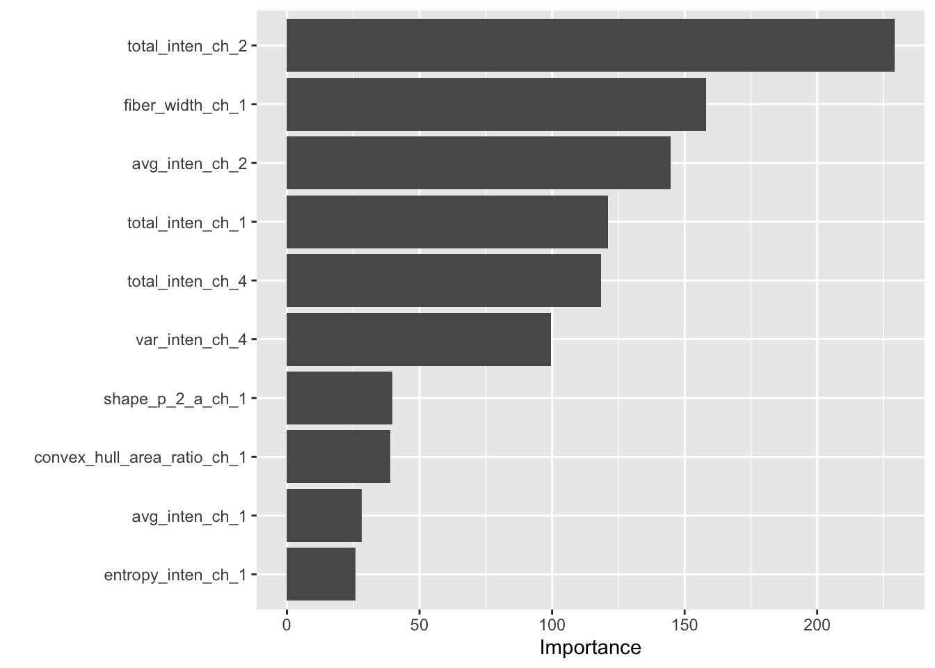
best_tree = tree_res.best_estimator_.named_steps['decisiontreeclassifier']
ct = tree_res.best_estimator_.named_steps['columntransformer']

feature_importances = pd.DataFrame({'name': ct.transformers_[0][2]}) \
    .assign(importance = best_tree.feature_importances_) \
    .sort_values('importance', ascending=False)

import seaborn as sns
sns.barplot(x='importance', y='name', data=feature_importances.head(10))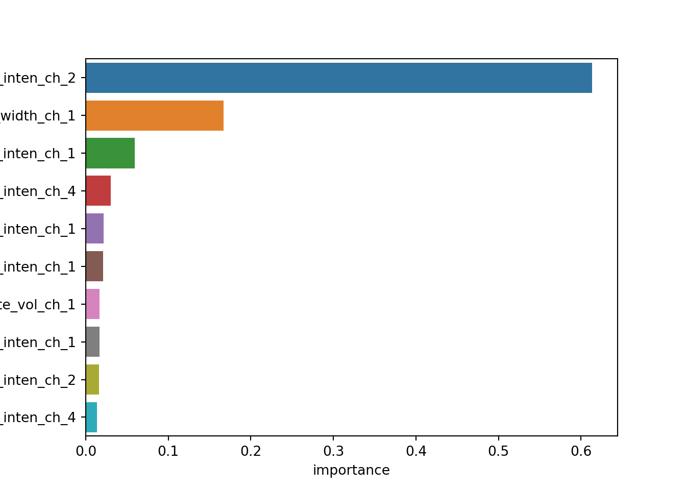
Final validation
best_tree %>%
  last_fit(cell_split) %>%
  collect_metrics()
## # A tibble: 2 x 3
## .metric .estimator .estimate
## <chr> <chr> <dbl>
## 1 accuracy binary 0.813
## 2 roc_auc binary 0.853pd.DataFrame.from_records([
(name, scorer(tree_res.best_estimator_, X_test, y_test))
for name, scorer in tree_scorer.items()
], columns=['metric', 'score'])## metric score
## 0 roc_auc 0.824385
## 1 accuray 0.776238