Introduction
I want this post to be an introduction to cleaning and preparing a messy spreadsheet as part of a data science pipeline. Instead of presenting a final product, I’d like to emphasize exploration as a natural part of tidying. My approach will follow Hadley Wickham’s tidy data principles outlined in his tidy data paper. At the end, our data should satisfy these three characteristics:
- one variable per column
- one observation per row
- each type of observational unit forms a table
Why Tidy?
In educational environments, data is often served in a format convenient for statistical algorithms. The student can apply an array of methods and try to derive some insight. But as Hadley explains in his paper, the reality is that the data scientists spend 80% of their time preparing data, and only 20% on the analysis itself. In his article, Hadley identifies tidy data as data that is ready to be analyzed by statistical programs. That’s our goal here.
The Data
I’ll be tidying Greg Nuckol’s spreadsheet of periodization studies on strength training found on his website Strong By Science. I choose this dataset because Greg shared it and encouraged others to analyze it, which I think is awesome. In a future blog post, I am going to conduct a Bayesian meta-analysis of this data and share my results.
To be clear, the phrase “cleaning the dataset” is non-judgmental and I’m not trying to pick on Greg. When building this spreadsheet, Greg had more important things to do than to make it friendly for computers, especially when tidy data can sacrifice human readability and has various other trade-offs.
I think these sorts of exercises develop fundamental skills for the aspiring data science and I thought I would contribute my own example. I commend Greg’s own analysis and his willingness to share his data, and I’m happy to go through the exercise of cleaning it up.
Follow Along
The original data (downloaded 1/13/18 from Greg’s website), the R script used to clean it, and the final tidy data can all be found in the Github repo I created to analyze Greg’s work.
I would encourage you download the data and follow along as I tidy up.
Cleaning
Before we start coding, we actually need to look at the data. Since Greg shared his data on Google sheets, this was my first glimpse.
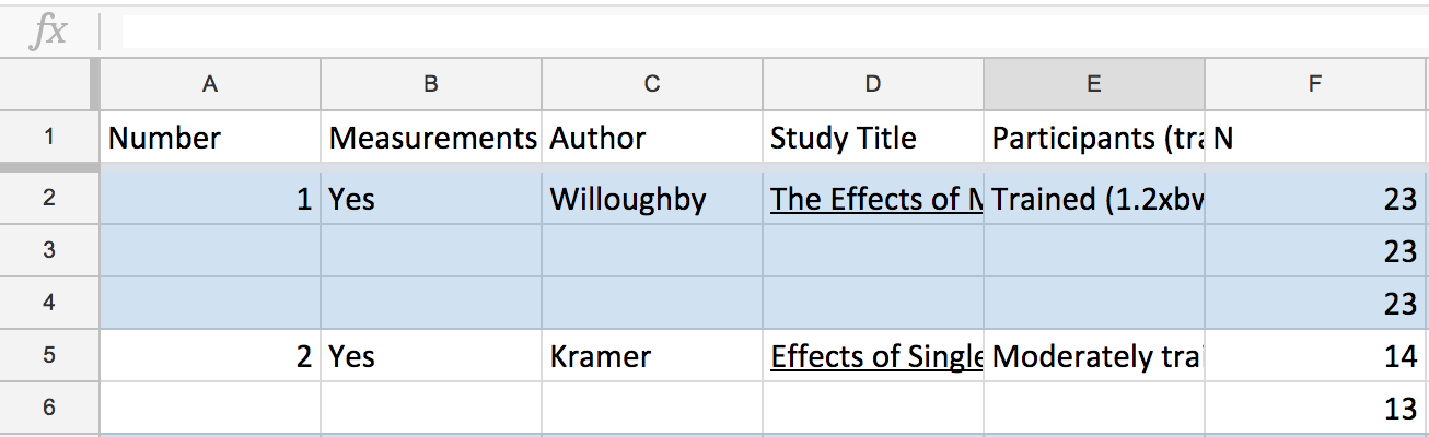
Greg has only filled out the study’s details for it’s first occurrence in the spreadsheet. This makes it easy to read by adding white space between each study, but hard for the computer because there is an implicit spatial relation, which makes grouping and lookups difficult.
Luckily, we can easily correct this spatial dependence:1 the first five variables always inherit the data from the previous row. We can code that as follows:
library(tidyverse)
library(magrittr)
d <- readxl::read_excel('Periodization Stuff.xlsx')
for (i in 1:nrow(d)) {
if (is.na(d[i,1])) {
d[i, c(1, 2, 3, 4, 5)] = d[i - 1, c(1, 2, 3, 4, 5)]
}
}Next, we need to make sure our import from Excel to R was successful. I suggest printing the data frame in various ways. Here, I noticed that one column (mostly) full of numbers was read as a character vector.
is.numeric(d$`Other 1 pre`)## [1] FALSEis.character(d$`Other 1 pre`)## [1] TRUEManually looking through the data I see that there is a URL (accidentally?) stored in what should be a numeric variable:
d[67,70]## # A tibble: 1 x 1
## `Other 1 pre`
## <chr>
## 1 https://www.dropbox.com/s/kyqean4j8zlfae9/Screenshot%202017-06-19%2009.…But we can coerce our vector to numeric, which changes any characters to NAs.
d$`Other 1 pre` <- as.numeric(d$`Other 1 pre`)Whenever I’m exploring a dataset and figuring out how to clean it, I use filters and head all the time. An easy way to improve the appearance of the console output is by hiding some of the less critical, text heavy columns using dplyr::select:
d %<>%
  select(
    -`Measurements at 3+ time points?`, -Author, -`Study Title`,
    -`Participants (training status)`, -Age, -Sex, -`Length (weeks)`,
    -`Intensity Closest to 1RM test`, -`Volume Equated?`, -Issues)
This makes the output more manageable and informative. Run this early in your pipeline and either delete or comment it out when you are finished so you can preserve all the data.
Next, you should notice that the last 70 columns are all numeric, with names such as squat, bench, LBM, etc. This violates the second principle of tidy data: we should have one observation per row. Instead, we have one program type (per study) per row, with multiple observations (squat, bench, LBM, etc) for each program type as columns. We need to gather the columns into one row:
d %<>%
  gather(type, outcome, `LBM Pre`:`ES 1 vs. 3__4`)
Let’s take a closer look at the variables we’ve gathered:
unique(d$type)## [1] "LBM Pre" "LBM SD"
## [3] "LBM post" "% increase"
## [5] "ES pre/post" "ES 1 vs. 2, 2 vs. 3"
## [7] "ES 1 vs 3" "MT Pre"
## [9] "MT SD" "MT Post"
## [11] "% increase__1" "ES pre/post__1"
## [13] "ES 1 vs. 2, 2 vs. 3__1" "ES 1 vs 3__1"
## [15] "CSA pre" "CSA SD"
## [17] "CSA post" "% increase__2"
## [19] "ES pre/post__2" "ES 1 vs. 2, 2 vs. 3__2"
## [21] "ES 1 vs 3__2" "BF% pre"
## [23] "BF% SD" "BF% post"
## [25] "% increase__3" "ES pre/post__3"
## [27] "ES 1 vs. 2, 2 vs. 3__3" "ES 1 vs 3__3"
## [29] "Fiber CSA pre" "Fiber CSA SA"
## [31] "Fiber CSA post" "% increase__4"
## [33] "ES pre/post__4" "ES 1 vs. 2, 2 vs. 3__4"
## [35] "ES 1 vs 3__4" "Squat pre"
## [37] "Squat SD" "Squat post"
## [39] "% increase__5" "ES pre/post__5"
## [41] "ES 1 vs. 2/2 vs. 3" "ES 1 vs. 3"
## [43] "Bench Pre" "Bench SD"
## [45] "Bench post" "% increase__6"
## [47] "ES pre/post__6" "ES 1 vs. 2/2 vs. 3__1"
## [49] "ES 1 vs. 3__1" "Leg press pre"
## [51] "Leg press SD" "Leg press post"
## [53] "% increase__7" "ES pre/post__7"
## [55] "ES 1 vs. 2/2 vs. 3__2" "ES 1 vs. 3__2"
## [57] "Other 1 pre" "Other 1 SD"
## [59] "Other 1 post" "% increase__8"
## [61] "ES pre/post__8" "ES 1 vs. 2/2 vs. 3__3"
## [63] "ES 1 vs. 3__3" "Other 2 pre"
## [65] "Other 2 SD" "Other 2 post"
## [67] "% increase__9" "ES pre/post__9"
## [69] "ES 1 vs. 2/2 vs. 3__4" "ES 1 vs. 3__4"Okay, first we can safely ignore anything with “ES”2 or “%” in the name. Those are calculated, not observed quantities.
Now I see a pattern in the rest of the column names. Each outcome is named something like “[LBM/Bench/Squat] [Pre/Post/SD]”. This means we actually have two different variables in one column, which violates the first tidy principle: one variable per column. We need to separate the columns so we have a variable for outcome types such as LBM, bench, squat, etc. and outcome measurements such as pre, post, and SD:
d %<>%
  mutate(type = str_to_lower(type)) %>%
  filter(
    (str_detect(type, ' pre') |
    str_detect(type, ' post') |
    str_detect(type, ' sd')) &
    not(str_detect(type, "/"))) %>%
  separate(
    type, c('outcome_type', 'outcome_measurements'),
    ' (?=(pre$|post$|sd$))')
This gives us
head(d %>% select(Number, outcome_type, outcome_measurements, outcome))## # A tibble: 6 x 4
## Number outcome_type outcome_measurements outcome
## <dbl> <chr> <chr> <chr>
## 1 1.00 lbm pre <NA>
## 2 1.00 lbm pre <NA>
## 3 1.00 lbm pre <NA>
## 4 2.00 lbm pre 66.5
## 5 2.00 lbm pre 68.9
## 6 3.00 lbm pre <NA>As we can see, study number one didn’t measurement LBM. We only care what each study did measure, so we can now remove all the NAs and change outcome to numeric.
d <- d[complete.cases(d$outcome),]
d$outcome <- as.numeric(d$outcome)
Now, let’s narrow our attention to study number one. When in doubt, start small.
head(d %>% filter(Number == 1) %>% select(-`Program Details`))## # A tibble: 6 x 6
## Number N `Program Label` outcome_type outcome_measurements outcome
## <dbl> <dbl> <chr> <chr> <chr> <dbl>
## 1 1.00 23.0 NP squat pre 1.48
## 2 1.00 23.0 NP squat pre 1.48
## 3 1.00 23.0 LP/BP squat pre 1.48
## 4 1.00 23.0 NP squat sd 0.105
## 5 1.00 23.0 NP squat sd 0.105
## 6 1.00 23.0 LP/BP squat sd 0.105Taking a closer look at the new columns, I would contend that the outcome_measurements columns now violates principle one: one variable per column. For comparison, outcome_type is definitely one variable. It indicates what the study was actually measuring as an outcome. But outcome_measurements is a collection of three different variables, pre, post, and sd that measure some aspect of the outcome_type. Therefore, we need to separate into their own column.
Let’s look at all the relevant data for study one.
d %>% filter(Number == 1) %>% select(-N, -Number)## # A tibble: 18 x 5
## `Program Label` `Program Details` outcome_type outcome_measure… outcome
## <chr> <chr> <chr> <chr> <dbl>
## 1 NP 5x10RM (78.9%); … squat pre 1.48
## 2 NP 6x8RM (83.3%); w… squat pre 1.48
## 3 LP/BP 5x10RM for 4 wee… squat pre 1.48
## 4 NP 5x10RM (78.9%); … squat sd 0.105
## 5 NP 6x8RM (83.3%); w… squat sd 0.105
## 6 LP/BP 5x10RM for 4 wee… squat sd 0.105
## 7 NP 5x10RM (78.9%); … squat post 1.74
## 8 NP 6x8RM (83.3%); w… squat post 1.89
## 9 LP/BP 5x10RM for 4 wee… squat post 2.02
## 10 NP 5x10RM (78.9%); … bench pre 1.28
## 11 NP 6x8RM (83.3%); w… bench pre 1.28
## 12 LP/BP 5x10RM for 4 wee… bench pre 1.28
## 13 NP 5x10RM (78.9%); … bench sd 0.00200
## 14 NP 6x8RM (83.3%); w… bench sd 0.00200
## 15 LP/BP 5x10RM for 4 wee… bench sd 0.00200
## 16 NP 5x10RM (78.9%); … bench post 1.41
## 17 NP 6x8RM (83.3%); w… bench post 1.43
## 18 LP/BP 5x10RM for 4 wee… bench post 1.60If we read closely, we can see that there were three unique protocols in study one. Each protocol has a unique pre, post, and sd measurement. We can exploit that grouped structure3 by dividing the data into those groups and then spreading the outcome_measurements to a column containing the numeric outcome.
d %>%
  filter(Number == 1) %>%
  select(-N, -Number) %>%
  mutate_if(is.character, funs(factor(.))) %>%
  group_by(
    `Program Label`, `Program Details`, outcome_type, outcome_measurements) %>%
  spread(outcome_measurements, outcome)
## # A tibble: 6 x 6
## # Groups: Program Label, Program Details, outcome_type [6]
## `Program Label` `Program Details` outcome_type post pre sd
## * <fct> <fct> <fct> <dbl> <dbl> <dbl>
## 1 LP/BP 5x10RM for 4 weeks, 4x… bench 1.60 1.28 0.00200
## 2 LP/BP 5x10RM for 4 weeks, 4x… squat 2.02 1.48 0.105
## 3 NP 5x10RM (78.9%); weight… bench 1.41 1.28 0.00200
## 4 NP 5x10RM (78.9%); weight… squat 1.74 1.48 0.105
## 5 NP 6x8RM (83.3%); weights… bench 1.43 1.28 0.00200
## 6 NP 6x8RM (83.3%); weights… squat 1.89 1.48 0.105This works perfect4. Let’s apply it to the rest of the data set (remembering to include the study number):
d %<>%
  mutate_if(is.character, funs(factor(.))) %>%
  group_by(
    outcome_type, outcome_measurements, Number, `Program Label`, `Program Details`) %>%
  spread(outcome_measurements, outcome) %>%
  ungroup()
## Error: Duplicate identifiers for rows (114, 115), (120, 121, 122, 123), (90, 91), (96, 97, 98, 99), (102, 103), (108, 109, 110, 111)We got an error, but we can work with this. It tells us where spread sees identical groups. This is most likely missing data, which tells us not every study is organized as nicely study one.
d[c(114, 115, 120, 121, 122, 123, 90, 91, 96, 97, 98, 99, 102, 103, 108, 109, 110, 111),]## # A tibble: 18 x 7
## Number N `Program Label` `Program Details` outcome_type
## <dbl> <dbl> <chr> <chr> <chr>
## 1 35.0 NA <NA> <NA> mt
## 2 35.0 NA <NA> <NA> mt
## 3 47.0 NA <NA> <NA> mt
## 4 47.0 NA <NA> <NA> mt
## 5 47.0 NA <NA> <NA> mt
## 6 47.0 NA <NA> <NA> mt
## 7 35.0 NA <NA> <NA> mt
## 8 35.0 NA <NA> <NA> mt
## 9 47.0 NA <NA> <NA> mt
## 10 47.0 NA <NA> <NA> mt
## 11 47.0 NA <NA> <NA> mt
## 12 47.0 NA <NA> <NA> mt
## 13 35.0 NA <NA> <NA> mt
## 14 35.0 NA <NA> <NA> mt
## 15 47.0 NA <NA> <NA> mt
## 16 47.0 NA <NA> <NA> mt
## 17 47.0 NA <NA> <NA> mt
## 18 47.0 NA <NA> <NA> mt
## # ... with 2 more variables: outcome_measurements <chr>, outcome <dbl>As expected, lots of missing data. Seemingly important data such as Program Label, Details, and participants. There is a temptation to toss it out, but only studies 35 and 47 are missing this data. We can easily go back to the source and see what’s going on.
Referring back to the original data, it looks like the missing data is a strange encoding of some smaller muscles like elbow flexors and triceps. I’m going to exclude it, because it would probably take some manual data manipulation to fix. Also, in the next blog post I’m going to focus on the squat and bench so it won’t matter in the long run.
So let’s try it without those rows:
d <- d[-c(114, 115, 120, 121, 122, 123, 90, 91, 96, 97, 98, 99, 102, 103, 108, 109, 110, 111),]d %<>%
mutate_if(is.character, funs(factor(.))) %>%
group_by(
outcome_type, outcome_measurements, Number, `Program Label`, `Program Details`) %>%
spread(outcome_measurements, outcome) %>%
ungroup()And we have no errors!
Final Product
We could call write.csv on our dataset right now and be done with it. The data would be shareable, but the process isn’t very repeatable. Not only that, but our dataset would be incomplete. Remember we deleted a bunch of columns with dplyr:select to make it easier to see on the command line.
For these reasons, I would encourage you to translate your interactive commands into a standalone .R script that exists in an isolated environment only containing the original data, such as the one I made for this blog post. The isolated environment eliminates forgotten dependencies in the interactive working environment, an .R script solves the repeatibility problem, and posting on Github improves our sharing.
Conclusion
Figuring out how to clean a dataset should be interactive and exploratory. Trying things out and getting error messages points you in the next direction. Don’t wring your hands: start small. But simultaneously, save what works. Iterate on what you have. And keep the exploration environment and product environment separate so you aren’t afraid to break things, and you have a baseline to return to when you do.
This synergy between exploration and iteration is universal in data science, and it was fun to share it with you in this blog post.
Sometimes we can’t easily fix spatial relations. For example, Excel pivot tables are notorious for the complicated use of whitespace and empty cells. For more advanced spreadsheet munging, check out tidyxl package.↩
ES stands for effect size. We’ll talk about that in the next blog post↩
mutate_if(is.character, funs(factor(.))) %>%transforms each character column to a factor column for easy grouping. I believer-basedata frames do this automatically, but eitherreadxlortibbledoesn’t.↩